Code
dag_nomiss <- dagify(
  Y ~ X + Z1 + Z2,
  X ~ Z1 + Z2 + U,
  Z1 ~ U,
  Z2 ~ U,
  coords = list(
    x = c(U = 0.75, Z1 = 1, Z2 = 1, X = 2, Y = 3),
    y = c(U = 0, Z1 = 1, Z2 = -1, X = 0, Y = 0)
  )
)
ggdag(dag_nomiss) + theme_dag()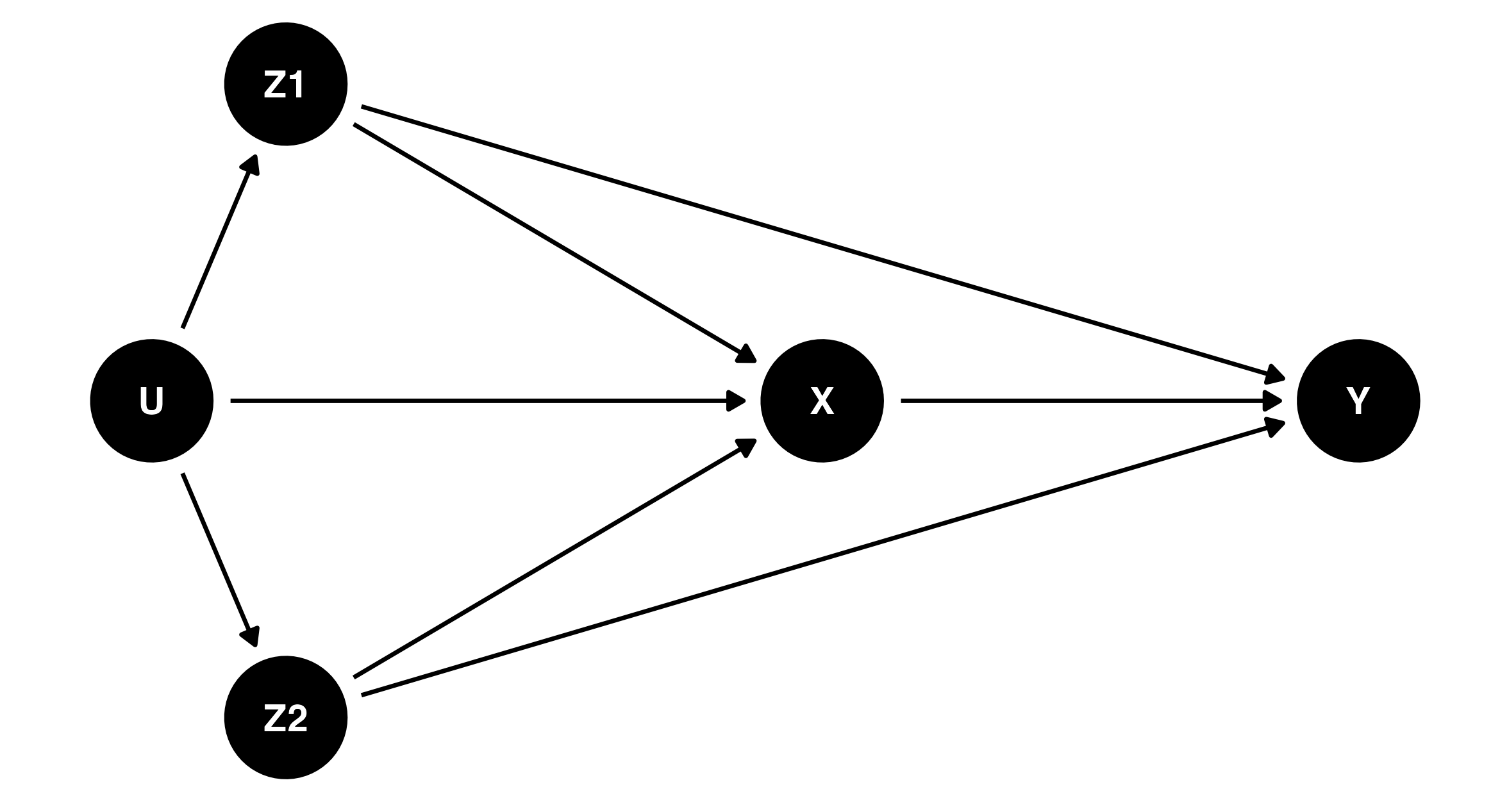
Missing data refers to data which was intended to have been collected but was not, and is a common scenario in biomedical and social science research. Analysing datasets that have missing data requires extra care and consideration to produce correct results.
The best method for dealing with missing data depends on the underlying process causing the missingness. There is no single approach that is always the best, and the terminology commonly used to describe missingness doesn’t directly relate to what analysis methods perform best. In this blog post I’ll begin by defining the commonly used but sometimes unhelpful classifications for missing data mechanisms (you’ll see them everywhere, so you might as well know what they mean) and then explain how to describe missing data processes using causal diagrams (DAGs) and provide some references to help choose an analysis based on that.

The most common classification for missing data mechanisms is that data is either Missing Completely at Random (MCAR), Missing at Random (MAR), or Missing Not at Random (MNAR). This classification is based on concepts first introduced in Rubin (1976). These terms are widespread, but can be confusing when first encountered because they do not mean quite what you might expect them to mean. I’ll define them briefly here, but the goal is to not have to focus specifically about which of these mechanisms apply to your data, or use this classification to guide your analytical choices.
Data is considered to be Missing Completely at Random (MCAR) if the probability of being missing does not depend on the values of any of the variables in the data, whether those values are missing or observed (Little & Rubin, 2014, p. 12). In other words, the missingness cannot be related to the research question of interest (Lee et al., 2021).
Data is Missing at Random (MAR) if the probability of being missing depends only on data that was observed (Little & Rubin, 2014, p. 12). Most commonly this refers to a situation where a variable with incomplete data has probability of being missing which relates to completely-observed variables, but there are other possibilities which fit this definition too1. This term is misleading if encountered without context, as a plain-language interpretation suggests it may mean something more like MCAR. However, MCAR is a stricter requirement than MAR. If data is MCAR, it is also considered MAR.
Data is Missing Not at Random (MNAR) if it’s not Missing at Random (Little & Rubin, 2014, p. 12). At least that’s relatively straightforward. In other words, the probability of data being missing is related to what the missing values would have been, had we observed them. It is sometimes implied that MNAR data is a lost cause for statistical analysis, but later in this post we will see specific examples of MNAR mechanisms where common statistical procedures produce valid results for common questions.
Strictly speaking, these classifications refer to the entire dataset collectively, usually consisting of many variables, some of which may have missing values and some of which may not. When there are multiple variables with missing values — a common situation in real datasets — these classifications are sometimes informally applied to specific variables with missing data, but doing so doesn’t relate to any of the mathematical guarantees about which analysis methods are applicable.
These missing data classifications depend on the type of analysis and set of available variables. For example, if additional variables (sometimes called auxiliary variables) which relate to probability of partially-observed variables having missing values are added to the dataset, the missing data mechanism may change from being MNAR to being MAR.
Rubin (1976) is often cited as the source of this classification system, but didn’t actually introduce the terms Missing Completely at Random or Missing Not at Random, only Missing at Random. Rubin originally defined an additional condition, Observed at Random. Data which is both Missing at Random and Observed at Random is what we would now commonly refer to as Missing Completely at Random. The term Missing Completely at Random came later, in Marini et al. (1980). This history is given in Little (2021) and was also confirmed in a Tweet by Raphael Nishimura: ‘I was curious about that too and did some digging with the authors. Rod said that “Rubin’s 1976 Biometrika paper defines MAR and OAR (observed at random) but he may not have put the two together.” Don confirmed it and added that “MCAR was first formally defined in a joint paper with Marini and Olsen, I think in 1980, in a more applied paper.”’
Sometimes you may hear missing data described as “ignorable” or “non-ignorable”. These terms are also potentially misleading. “Ignorable” missing data doesn’t mean that you can just ignore the fact that you have missing data when doing an analysis. This term was defined in Rubin (1976) to mean that (1) the data is MAR; (2) the likelihood can be factorised into a part relating to the missingness probability and a part relating to the distribution of the underlying data. These provide a sufficient condition for missing data to be dealt with using likelihood-based methods.
Unfortunately, there’s no way to determine the missing data mechanism purely by looking at the data — you need to think about the process generating the data and why some of it is missing. Often there will be different reasons for missing data in the same variable. A causal DAG is a good way to reason about the relationship between the variables and their reasons for being missing and can help you decide what analysis to use. Rather than using the DAG to determine whether your data is MCAR, MAR, or MNAR, and then use those classifications to choose an analysis, you can use the DAG directly to guide your choice of analysis method. I’ll have examples of this later in this blog.
It depends! (I’m a statistician, you should have known I would say that.) These are the standard results about what missing data methods are appropriate under different processes:
Complete case analysis is unbiased if the data is MCAR. This is a sufficient condition, not a necessary condition (Little, 2021): there are situations where complete case analysis may be valid, or at least provide a valid estimate of a particular quantity of interest, under MAR or MNAR. Depending on the amount of missing data, complete case analysis may be inefficient (i.e., have lower power than other methods) because only cases where no variables have missing values are used in the analysis.
Multiple imputation, inverse probability weighting, likelihood-based methods and full Bayesian methods are unbiased if the data is MAR or MCAR (Little, 2021). Multiple imputation is approximately equivalent to a maximum-likelihood method if the underlying model is the same (Collins et al., 2001).
In some specific MNAR situations, some of the above methods may still be valid, depending on what you’re trying to estimate (White & Carlin, 2010).
To make these definitions more concrete, here are some examples of missing data mechanisms that may occur in real studies.
Sometimes missing data arises from a study design where some data is not collected on some participants. For example, consider a psychometric instrument with a large number of items. The items could be split up into sets which are asked at different times; for example, half at baseline and half a follow-up. Ideally this process would be randomised so each participant receives a different random split. The items which were not asked at a particular time point are missing values, and because the missingness was deliberately introduced by the experimenter using randomisation, we know that the probability of a particular item being missing is unrelated to any other variable in the study.
This is one of the few cases where we can be sure the data is MCAR.
Causal diagrams are used to represent causal relationships between variables in a study (Pearl, 1995). These relationships are shown visually using a directed acyclic graph (DAG), which is a mathematical term for a bunch of circles with arrows between them. The circles (nodes) represent variables and arrows (edges) between them represent direct causal pathways. The direction of the arrows represents the direction of causation, and a valid DAG never has a path leading from a particular point back to that same point2. If there is no path following the arrows between two variables in a DAG, there is no causal connection between them.
The structure of the DAG behind your data cannot be inferred just from looking at the data. It needs to come from substantive expertise about the underlying variables in the data, their relationship to each other, and how the data was collected.
The idea of using a DAG to represent missing data assumptions was first introduced in Mohan & Pearl (2014). To provide more practical advice for specific scenarios, Moreno-Betancur et al. (2018) introduces “canonical” causal diagrams for missing data in the setting where we want to estimate the relationship between an outcome Y and an exposure X3, adjusting for some confounding variables which may influence both the outcome and the exposure. The confounding variables may be either completely observed (Z1) or have some missing data (Z2). There may also be some unknown, unmeasured factors U which affect the exposure and the confounders.
The DAG corresponding to the scenario above is shown below. If you click the “Code” button you can see how it was produced in R, using the packages dagitty (Textor et al., 2017) and ggdag. You don’t need to understand R code to use and apply DAGs but it is provided as an example for those who may want to make causal diagrams for their own studies. The first part of the code describes the underlying relationships between the variables, using the same syntax used to describe regression models in R. The second part of the code sets up the visual coordinates used for plotting the DAG — an aesthetic consideration only.
dag_nomiss <- dagify(
Y ~ X + Z1 + Z2,
X ~ Z1 + Z2 + U,
Z1 ~ U,
Z2 ~ U,
coords = list(
x = c(U = 0.75, Z1 = 1, Z2 = 1, X = 2, Y = 3),
y = c(U = 0, Z1 = 1, Z2 = -1, X = 0, Y = 0)
)
)
ggdag(dag_nomiss) + theme_dag()
This DAG is called a complete-data DAG, or c-DAG. It represents the causal relationships between the variables if all of them had been completely observed.
To represent possible causes of missing data, we can introduce three new variables in the DAG: MX, MY and MZ2, representing whether or not the exposure (X), outcome (Y), or partially-observed confounders (Z2) are missing. Think of them as binary indicator variables, where for example MX = 1 means that X wasn’t observed (for a particular case/participant/observation) and MX = 0 means that X was observed. Adding these variables produces a missingness DAG, or m-DAG. Moreno-Betancur et al. (2018) also considers unmeasured causes of missingness (W) which are not related to any of the substantive variables in the study but do affect the probability of missingness.
The variables in the DAG which aren’t prefixed with M still refer to values of the variables as if they had been completely observed — which we no longer have full access to in our real data since we only get to see the variables after the missingness mechanism has occurred. This ensures that the causal mechanism in the c-DAG still applies to the m-DAG, so the m-DAG can be produced by adding additional nodes and arrows to the c-DAG without changing any of the arrows between existing nodes.
If we turn the c-DAG above into an m-DAG by adding nodes for MX, MY, and MZ2 but no additional arrows, the absence of arrows to MX, MY and MZ2 would mean that there is no causal relationship between any of the variables and their missingness — in other words, the MCAR missingness mechanism. This scenario would be quite unusual in most real studies, unless the missing data was deliberately planned like our first example in the previous section.
This m-DAG is shown below, with an additional variable W representing unmeasured variables which affect the missing data process but are not related to any of the variables in the study. The new variables representing the missing data mechanism are shown in blue. In that MCAR scenario, the blue nodes (missing data mechanism) are completely disconnected from black nodes (relating to the main research question).
dag_mcar <- dagify(
  Y ~ X + Z1 + Z2,
  X ~ Z1 + Z2 + U,
  Z1 ~ U,
  Z2 ~ U,
  MX ~ W,
  MY ~ W,
  MZ2 ~ W,
  coords = list(
    x = c(U = 0.75, Z1 = 1, Z2 = 1, X = 2, Y = 3,
          MX = 1.5, MY = 2, MZ2 = 2.5, W = 2),
    y = c(U = 0, Z1 = 0.75, Z2 = -0.75, X = 0, Y = 0,
          MX = 1.75, MY = 1.75, MZ2 = 1.75, W = 2.5)
  )
)
dag_mcar %>%
  tidy_dagitty() %>%
  mutate(
    node_colour = case_when(
      str_starts(name, "M") | name == "W" ~ "dodgerblue3",
      .default = "black"
    ),
    edge_colour = case_when(
      str_starts(to, "M") ~ "dodgerblue3",
      .default = "black"
    )
  ) %>%
  ggplot(aes(x = x, y = y, xend = xend, yend = yend)) +
  geom_dag_edges(aes(edge_colour = edge_colour)) +
  geom_dag_point(size = 16, aes(colour = node_colour)) +
  geom_dag_text(colour = "white", size = 3.88) +
  theme_dag() +
  scale_colour_identity()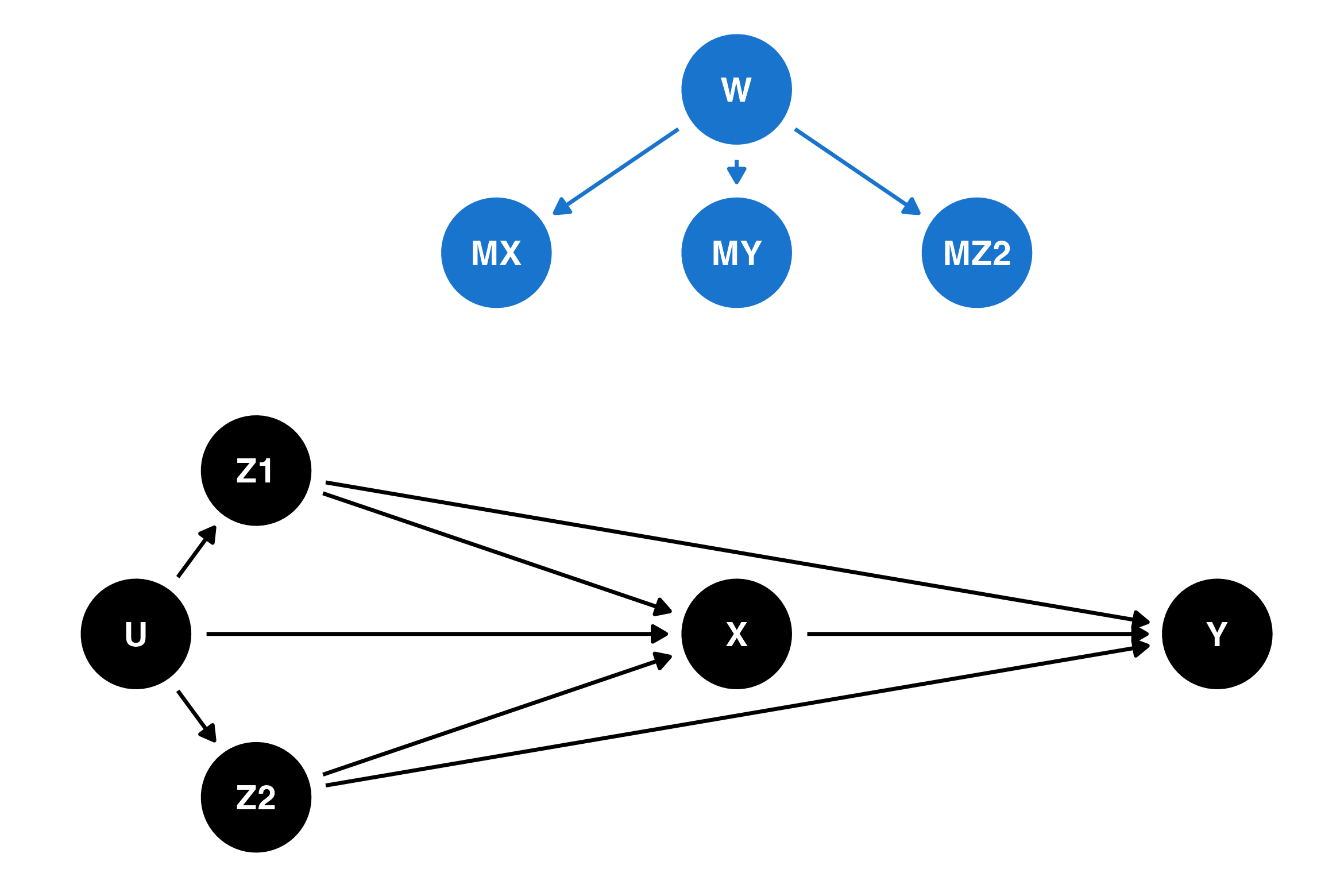
Figure 2 in Moreno-Betancur et al. (2018) provides 10 examples of m-DAGs, with different combinations of the following features:
The first of these canonical DAGs, m-DAG A, is an example of a MAR process, where the missingness is only related to completely-observed confounders (Z1) and unmeasured variables unrelated to other variables in the study (W). This DAG describes Example 2 in the previous section, with participant location (part of Z1) causing missingness in other variables (MX, MY, MZ2). This DAG is reproduced below, with the nodes and arrows related to the missing data mechanism shown in blue:
dag_a <- dagify(
  Y ~ X + Z1 + Z2,
  X ~ Z1 + Z2 + U,
  Z1 ~ U,
  Z2 ~ U,
  MX ~ Z1 + W,
  MY ~ Z1 + W,
  MZ2 ~ Z1 + W,
  coords = list(
    x = c(U = 0.75, Z1 = 1, Z2 = 1, X = 2, Y = 3,
          MX = 1.5, MY = 2, MZ2 = 2.5, W = 2),
    y = c(U = 0, Z1 = 0.75, Z2 = -0.75, X = 0, Y = 0,
          MX = 1.75, MY = 1.75, MZ2 = 1.75, W = 2.5)
  )
)
dag_a %>%
  tidy_dagitty() %>%
  mutate(
    node_colour = case_when(
      str_starts(name, "M") | name == "W" ~ "dodgerblue3",
      .default = "black"
    ),
    edge_colour = case_when(
      str_starts(to, "M") ~ "dodgerblue3",
      .default = "black"
    )
  ) %>%
  ggplot(aes(x = x, y = y, xend = xend, yend = yend)) +
  geom_dag_edges(aes(edge_colour = edge_colour)) +
  geom_dag_point(size = 16, aes(colour = node_colour)) +
  geom_dag_text(colour = "white", size = 3.88) +
  theme_dag() +
  scale_colour_identity()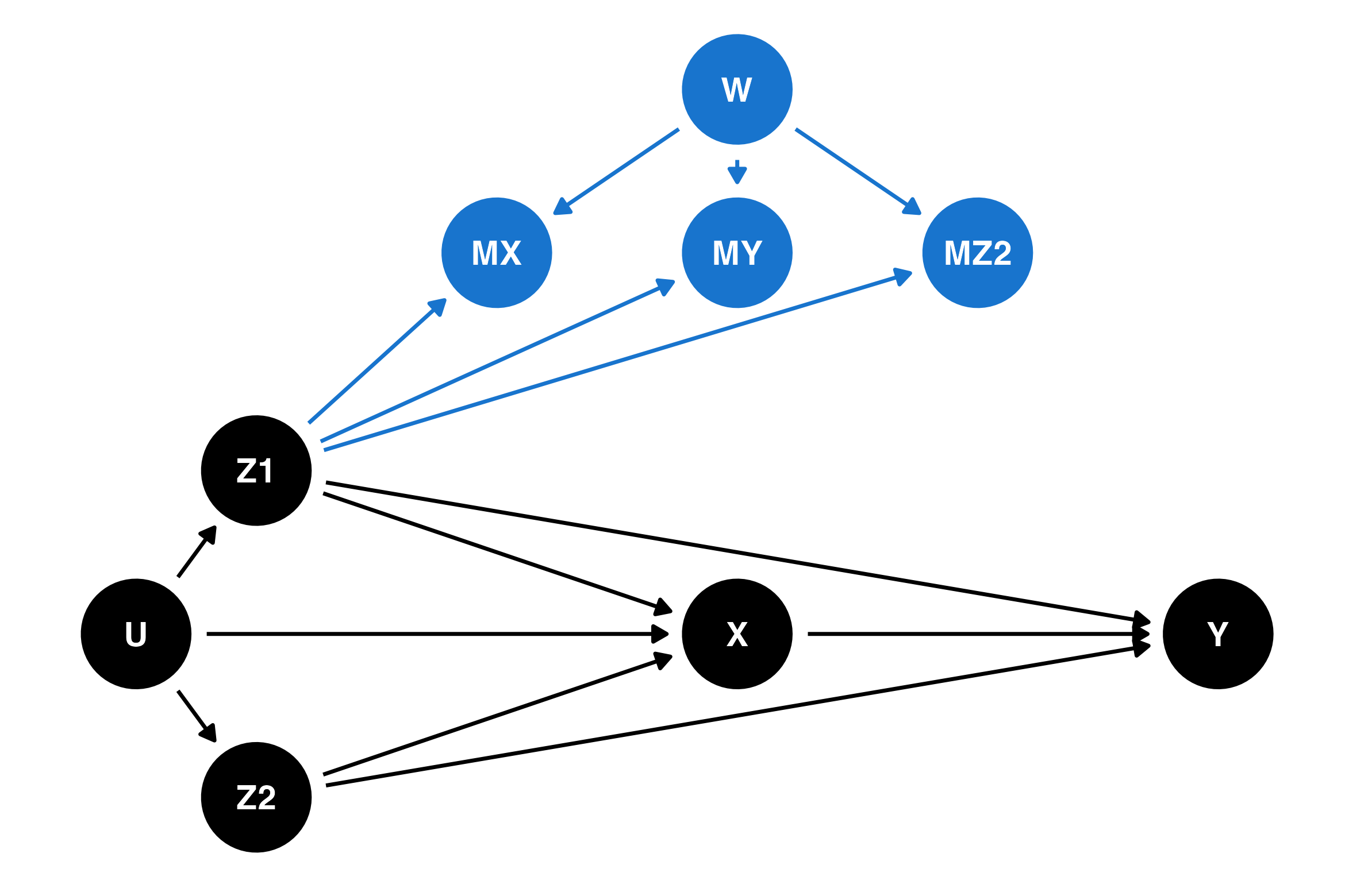
In this DAG, so long as the model’s adjustment for confounders is correctly specified (a big “if”!), both complete cases analysis and multiple imputation provide valid estimates of not just the relationship between the exposure and the outcome, but also the complete distribution of the outcome. This isn’t something that should be obvious just from looking at the DAG — there’s a derivation in the supplementary materials for Moreno-Betancur et al. (2018) for this and the other DAGs, with the results summarised in Tables 1 and 2 of that paper. Those who are familiar with causal DAGs may want to know that when there is missing data, this derivation is more complex than rules like “d-separation” and cannot be done algorithmically.
In other missing data situations, it may be possible to obtain a valid estimate of the effect of the exposure but not, for example, the population mean of the outcome. In some situations, it may not be possible to obtain a valid estimate of either.
The figure below shows m-DAG E, which is an example of an MNAR process. The arrows new to this DAG which weren’t in m-DAG A are shown in red. The probability of missingness in all variables is affected by both the exposure X (which may itself have missing values) and partially-observed confounders Z2. This DAG corresponds to Example 3 in the previous section, if we believe that missingness in child behaviour is not related to the missing values of child behaviour. Perhaps surprisingly, even though this missingness process is MNAR, it is possible to obtain a valid estimate of the relationship between the exposure and the outcome using either complete cases analysis or multiple imputation. However, it is not possible to recover the overall population mean of the outcome.
dag_e <- dagify(
  Y ~ X + Z1 + Z2,
  X ~ Z1 + Z2 + U,
  Z1 ~ U,
  Z2 ~ U,
  MX ~ Z1 + Z2 + X + W,
  MY ~ Z1 + Z2 + X + W,
  MZ2 ~ Z1 + Z2 + X + W,
  coords = list(
    x = c(U = 0.75, Z1 = 1, Z2 = 1, X = 2, Y = 3,
          MX = 1.5, MY = 2, MZ2 = 2.5, W = 2),
    y = c(U = 0, Z1 = 0.75, Z2 = -0.75, X = 0, Y = 0,
          MX = 1.75, MY = 1.75, MZ2 = 1.75, W = 2.5)
  )
)
dag_e %>%
  tidy_dagitty() %>%
  mutate(
    node_colour = case_when(
      str_starts(name, "M") | name == "W" ~ "dodgerblue3",
      .default = "black"
    ),
    edge_colour = case_when(
      str_starts(to, "M") & name %in% c("X", "Z2") ~ "firebrick3",
      str_starts(to, "M") ~ "dodgerblue3",
      .default = "black"
    )
  ) %>%
  ggplot(aes(x = x, y = y, xend = xend, yend = yend)) +
  geom_dag_edges(aes(edge_colour = edge_colour)) +
  geom_dag_point(size = 16, aes(colour = node_colour)) +
  geom_dag_text(colour = "white", size = 3.88) +
  theme_dag() +
  scale_colour_identity()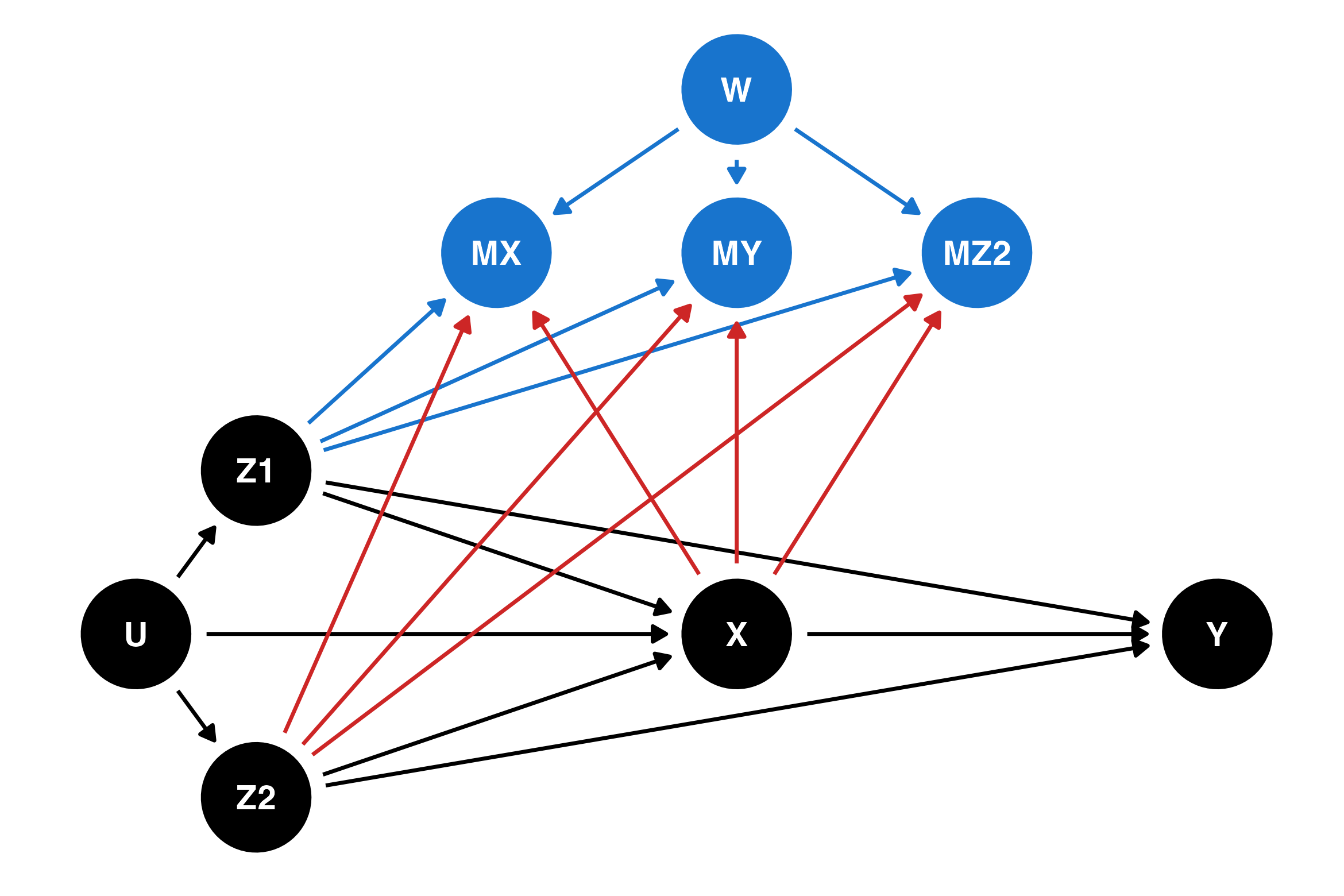
The final example in this blog is m-DAG J, which is another MNAR process. The arrows new to this DAG are shown in purple. In this example, missingness is also affected by the value of the outcome Y. This DAG is similar to the one for Example 3 in the previous section, if we believe that missingness in the outcome (child behaviour) is related to its own unobserved values. For this m-DAG, it is not possible to recover the relationship between the outcome and the exposure.
dag_j <- dagify(
  Y ~ X + Z1 + Z2,
  X ~ Z1 + Z2 + U,
  Z1 ~ U,
  Z2 ~ U,
  MX ~ Z1 + Z2 + X + Y + W,
  MY ~ Z1 + Z2 + X + Y + W,
  MZ2 ~ Z1 + Z2 + X + Y + W,
  coords = list(
    x = c(U = 0.75, Z1 = 1, Z2 = 1, X = 2, Y = 3,
          MX = 1.5, MY = 2, MZ2 = 2.5, W = 2),
    y = c(U = 0, Z1 = 0.75, Z2 = -0.75, X = 0, Y = 0,
          MX = 1.75, MY = 1.75, MZ2 = 1.75, W = 2.5)
  )
)
dag_j %>%
  tidy_dagitty() %>%
  mutate(
    node_colour = case_when(
      str_starts(name, "M") | name == "W" ~ "dodgerblue3",
      .default = "black"
    ),
    edge_colour = case_when(
      str_starts(to, "M") & name == "Y" ~ "darkorchid3",
      str_starts(to, "M") & name %in% c("X", "Z2") ~ "firebrick3",
      str_starts(to, "M") ~ "dodgerblue3",
      .default = "black"
    )
  ) %>%
  ggplot(aes(x = x, y = y, xend = xend, yend = yend)) +
  geom_dag_edges(aes(edge_colour = edge_colour)) +
  geom_dag_point(size = 16, aes(colour = node_colour)) +
  geom_dag_text(colour = "white", size = 3.88) +
  theme_dag() +
  scale_colour_identity()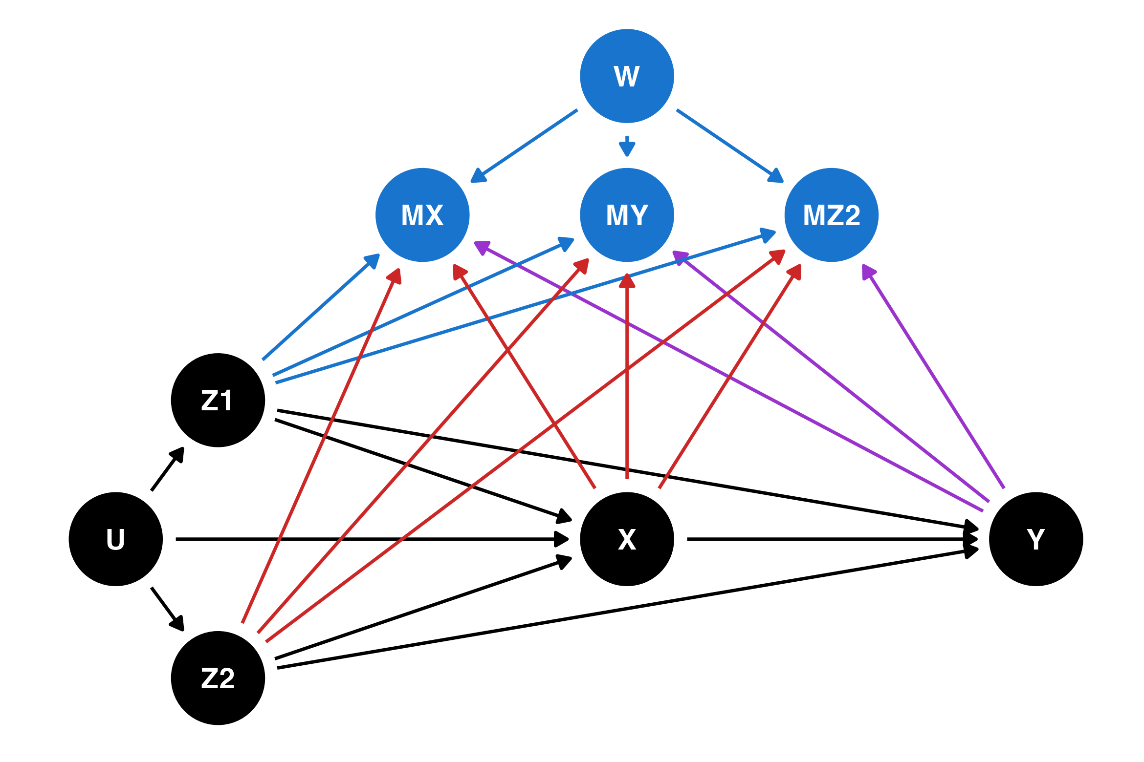
If you have an m-DAG where a quantity of interest cannot be recovered, you can consider doing a sensitivity analysis using a \(\delta\)-adjustment. This process is described in popular texts on missing data, e.g. van Buuren (2018) sec 9.2 (also available online) or Molenberghs et al. (2015).
This section draws heavily from Lee et al. (2023) — especially Figure 1 of that paper — which provides practical guidance for data analysis using missingness DAGs.
Start by determining the estimand of interest: the scientific quantity you would like to estimate, if you had access to the complete data.
Next, draw a DAG representing the causal relationships between your variables and their possible reasons for being missing. This will require some thinking about which arrows are plausible and which are not, based on your understanding of the real-world relationships between variables and the way the data has been collected.
Before deciding on an analysis method, you must first determine whether the estimand is recoverable, i.e. whether it is possible to estimate it from the data4. One possibility is to compare your DAG to the canonical DAGs in Moreno-Betancur et al. (2018) and the recoverability results in Table 1 of that paper.
If your estimand is recoverable, you can proceed to deciding on an analysis method to handle the missing data. Again, the canonical DAGs are useful for this. For canonical DAGs A, B, D and E, complete cases analysis was shown to provide a valid estimate of the relationship between the outcome and the exposure. For canonical DAGs A, B, C, D and E, multiple imputation was shown to provide a valid estimate of the relationship between the outcome and the exposure.
Randomised clinical trials provide some additional guarantees about the nature of the missing data process which observational studies do not: the assigned intervention is completely observed and known to be unrelated to baseline covariates. While it doesn’t use the m-DAG framework, Sullivan et al. (2018) considers several methods for dealing with missing data in randomised trials that may be useful for those working in that setting.
The papers above provide examples of situations where multiple imputation is not necessarily better than simpler methods, as well as situations where complete case analysis does not produce valid inference. The situations where particular missing data methods work do not neatly align with the definitions of MCAR/MAR/MNAR but by drawing a DAG and considering the results in the papers above you should be able to determine which popular methods are applicable to your data and research question.
Thanks to Isabella Ghement, Lachlan Cribb, and Tom Sullivan for providing valuable feedback which greatly improved this blog post. Last updated: 6 July 2023.
There are a few subtly different ways of defining this concept mathematically; Seaman et al. (2013) goes into the detail for those who are interested.↩︎
A “cycle” in mathematician-speak. Hence, directed (arrows have a direction) acyclic (can never get back to where you started) graph (set of nodes and edges).↩︎
That’s epidemiologist-speak for the main predictor of interest.↩︎
This step is analogous to determining identifiability in causal inference.↩︎